Simulating a Piano Soundboard

A 2D Finite Difference Time Domain Simulation

Author

Affiliation

Cam

Anauseam

With existing python libaries, it is not too difficult to simulate 2D acoustic wave propagation.

As a supporting document & python script for the Piano Acoustics & Tuning Report, this document will briefly cover the topic of simulating a piano soundboard over 2D space using the Finite Difference Time Domain (FDTD) method. This approach discretizes the continuous wave equation into a grid of points, allowing us to step through time and calculate the pressure at every point in the room.

The Physics Models

Unlike continuous time physics of the real world, computers must perform their calculations in discrete steps. Thus, we will have a small expose of discretizing the continuous wave equation for a 2D FDTD simulation.

The Continuous Wave Equation

The propagation of sound in a lossless 2D medium is governed by the 2D wave equation: \frac{\partial^2 u}{\partial t^2} = c^2 \left[ \nabla^2 u \right]

Where:

• u(x, y, t): Pressure (or displacement) of the air at a specific point.
• t: Time.
• c: Speed of sound (approx. 343 \text{ m/s}).
• \nabla^2: The Laplacian \nabla^2 = \frac{\partial^2}{\partial x^2} + \frac{\partial^2}{\partial y^2}, with \nabla^2 u representing the spatial curvature of the wave.

Discretizing the Equation (Finite Difference)

To solve this numerically, we not only need to discretize the equation for both space and time, but we also need to define how the physics changes from one time step to the next. This is done by solving for the future state of the system based on the current state and our physics model.

We begin by defining space as a grid of points such that u^n_{i,j} represents the pressure at spatial index (i, j) at time step n. Our goal is to solve for u^{n+1}_{i,j}, the pressure at the next time step, where n+1 is the next time step.

We start by approximating the derivatives using Central Finite Differences.

Time Derivative Approximation

The second derivative with respect to time is approximated as:

\frac{\partial^2 u}{\partial t^2} \approx \frac{u^{n+1}_{i,j} - 2u^n_{i,j} + u^{n-1}_{i,j}}{\Delta t^2}

where:

• u^{n+1}_{i,j}: Pressure at the next time step.
• u^n_{i,j}: Pressure at the current time step.
• u^{n-1}_{i,j}: Pressure at the previous time step.
• \Delta t: Time step size.

Spatial Laplacian Approximation

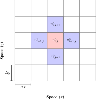
The 2D Laplacian is approximated by summing the differences between a point and its four nearest neighbors ¹ :

¹ The full finite difference formula for 2 dimensions is \nabla^2 u \approx \underbrace{\frac{u_{i+1,j} - 2u_{i,j} + u_{i-1,j}}{\Delta x^2}}_{\text{Curvature in } X} + \underbrace{\frac{u_{i,j+1} - 2u_{i,j} + u_{i,j-1}}{\Delta y^2}}_{\text{Curvature in } Y} However, because we assume a square grid where \Delta x = \Delta y, the formula simplifies to our formulation.

\nabla^2 u \approx \frac{u^n_{i+1,j} + u^n_{i-1,j} + u^n_{i,j+1} + u^n_{i,j-1} - 4u^n_{i,j}}{\Delta x^2}

Where:

• u^n_{i,j}: Pressure at the current space.
• u^n_{i+1,j}: Pressure at the space to the right.
• u^n_{i-1,j}: Pressure at the space to the left.
• u^n_{i,j+1}: Pressure at the space above.
• u^n_{i,j-1}: Pressure at the space below.
• \Delta x: Space step size

5-Point Stencil

NoteThe Five-Point Stencil

The choice of using the four nearest neighbors (plus the center point) is known as the 5-point stencil². It was chosen because it is the mathematical minimum required to represent 2D waves on a square grid symmetrically.

In the code, the Laplacian \nabla^2 u is calculated as:

\nabla^2 u \approx \frac{u_{left} + u_{right} + u_{up} + u_{down} - 4u_{center}}{\Delta x^2}

This is the standard Central Difference approximation. It looks at the immediate neighbors to determine if the center point is a “peak” (higher than neighbors) or a “valley” (lower than neighbors).

Why 5 points?

On a square grid, the 5-point stencil is the lowest order accurate stencil for the Laplacian. The reason is that we need enough information to approximate the second derivative (i.e. the curvature/acceleration).

• If you only look at 1 neighbor (e.g., right), you can only calculate the slope (first derivative), not the curvature.
• If you look at 2 neighbors (Left/Right), this gives you the curvature, but only along the X-axis. This would simulate a series of unconnected guitar strings (1D waves) running horizontally, but sound wouldn’t travel Up or Down.
• If you look at 3 neighbors, this would obviously be asymmetric.

To have a wave that travels in all directions (X and Y) on a square grid, you need at least one neighbor in every cardinal direction (+x, -x, +y, -y).

Higher Order Stencils

Although the 5-point stencil is the lowest order accurate stencil for the Laplacian, we absolutely could use a higher order stencil such as a 9-point stencil (diagonal neighbors included) or a 12-point stencil (including diagonals and neighbors of neighbors). This would be done because the 5-point stencil suffers from Numerical Dispersion:

• In the simple 5-point model, waves traveling along the diagonal axes (45 degrees) actually move at a slightly different speed than waves traveling along the grid lines (0 or 90 degrees). If you simulate a perfect explosion in the center, the expanding wave might look slightly like a diamond rather than a perfect circle.
• Including the diagonal neighbors (corner points) helps correct this “anisotropy,” making the wave propagation more perfectly circular (i.e. higher resolution).

As you can imagine, higher order stencils are more computationally expensive. For simple simulations such as this one, the 5-point stencil is sufficient.

² If you have any experience with signal or image processing, this is identical to a convolution operation. Specifically, it is the Laplacian Kernel used in image processing to detect edges. What physicists call the a stencil, signal processing engineers call a kernel (or even better, a filter).

The Final Difference Equation

Substituting the time derivative back into the wave equation:

\begin{align*} \frac{u^{n+1}_{i,j} - 2u^n_{i,j} + u^{n-1}_{i,j}}{\Delta t^2} &= c^2 \left[ \nabla^2 u \right] \\ u^{n+1}_{i,j} - 2u^n_{i,j} + u^{n-1}_{i,j} &= c^2 \Delta t^2 \left[ \nabla^2 u \right] \end{align*}

And isolating the future state u^{n+1}_{i,j}, we get:

u^{n+1}_{i,j} = \underbrace{2u^n_{i,j} - u^{n-1}_{i,j}}_{\text{Inertial Term}} + \underbrace{c^2 \Delta t^2 \left[ \nabla^2 u \right]}_{\text{Force Term}}

In this form we can analyze the behavior of the discretized system. Where:

• The Inertial Term represents momentum of the wave. If we assume the velocity is constant, the next position is just the current position plus the velocity times the time step.

\begin{align*} u_{next} &\approx u_{current} + (u_{current} - u_{previous})\\ &\approx 2u_{current} - u_{previous} \end{align*}

• The Force Term represents the effect of the wave on the medium. In this case, it’s the Laplacian of the pressure field, which models the diffusion of sound energy.

Expanding this further we can see other properties of the system and the update rule used in the code.

u^{n+1}_{i,j} = \underbrace{2u^n_{i,j} - u^{n-1}_{i,j}}_{\text{Inertial Term}} + \underbrace{\left( \frac{c \Delta t}{\Delta x} \right)^2}_{\text{Courant Number}} \underbrace{\left[ u^n_{i+1,j} + u^n_{i-1,j} + u^n_{i,j+1} + u^n_{i,j-1} - 4u^n_{i,j} \right]}_{\text{Discretized Laplacian}}

The Discrete Laplacian represents the restoring force, measuring the curvature of the wave.

• If the center point is higher than its neighbors (a peak), the result is negative, pulling the point down.
• If the center point is lower than its neighbors (a valley), the result is positive, pulling the point up. This is the mechanism that allows the wave to ripple outward; high points pull low neighbors up, and low neighbors pull high points down.

The Courant Number \frac{c \Delta t}{\Delta x} coefficient scales how strong the force is.

• This term dictates how far information can travel in one time step. If it’s too large (i.e. time step \Delta t is too long relative to grid spacing \Delta x), the simulation will become numerically unstable and “explode”.
• Because of this, the code calculatesdt using the CFL condition which dictates the maximum stable time step for a given grid spacing. In our case, we use a factor of 0.99 to ensure stability: dt = 1 / (C * np.sqrt(2) * (1 / dx)) * 0.99.

NoteThe CFL Condition

The CFL condition is formulated from the principle: Information cannot travel faster than the grid allows.

Consider the following scenario

A wave moving at speed c in one dimension. In one time step (\Delta t), the physical wave travels a distance of c \cdot \Delta t.

The wave must not skip over a grid point in a single step. The distance it travels (c \Delta t) must be less than or equal to the distance between grid points (\Delta x).

\begin{align*} \text{Distance Traveled} &\le \text{Grid Spacing}\\ c \Delta t &\le \Delta x \end{align*}

We can rearrange this to solve for the “Courant Number” (C), we get the 1D stability limit:

C = \frac{c \Delta t}{\Delta x} \le 1

If this ratio is greater than 1, a simulation is trying to move information further than one grid cell per step. The computer “misses” the interaction, errors accumulate, and the simulation crashes (values go to infinity).

Adapting to 2D

In our 2D simulation, waves don’t just travel along the X and Y axes; they travel diagonally. In a square grid, the distance between diagonal neighbors is \sqrt{\Delta x^2 + \Delta y^2}. If \Delta x = \Delta y, the diagonal distance is \Delta x\sqrt{2}. Thus for the standard 5-point stencil used in our 2D simulation, the mathematics of stability (specifically Von Neumann stability analysis) reveals that the sum of the Courant numbers in all dimensions must be less than 1. For a D-dimensional simulation, the condition becomes:

\frac{c \Delta t}{\Delta x} \le \frac{1}{\sqrt{D}}

Where D is the number of spatial dimensions (2 in this case).So, for a 2D simulation with a square grid, the strict limit is: \frac{c \Delta t}{\Delta x} \le \frac{1}{\sqrt{2}} \approx 0.707 This means you must take smaller time steps in 2D than in 1D to keep the simulation stable.

Python Implementation

Now that we have covered the theory, we can step through the Python code to cover the practical implementation. Recall that we will be simulating a vibrating piano soundboard. Although we have default values for the simulation, one can change them to see how they affect the simulation.

All the non-mathematical code is straight forward, and will not be covered in detail.

Configuration & Setup

To begin, the simulation is configured with the following parameters:

The Physics Engine

This section is the core of the simulation. It initializes an empty 2D grid and pressure states (e.g. u^n), and then enters a loop that updates the state of the grid over time.

Some brief notes on the code:

• A damping constant is made to ensure that the simulation does not become unstable due to floating point errors: damping = np.float32(0.995)
• The source is injected into the soundboard region and is constantely driven by a sine wave of a given frequency throughout the duration of the simulation: source_val = np.sin(2 * np.pi * FREQUENCY * (total_steps * dt))

Laplacian Operation

This is Laplacian Operator in our python code

```{python}
laplacian = (
    u[2:, 1:-1] +     # Right Neighbor (i+1)
    u[:-2, 1:-1] +    # Left Neighbor (i-1)
    u[1:-1, 2:] +     # Up Neighbor (j+1)
    u[1:-1, :-2] -    # Down Neighbor (j-1)
    4 * u[1:-1, 1:-1] # Center Point (i, j)
)
```

This is a purely vectorized operation, different from our orignally proposed iterative operation. Thus we will take a moment to explain the syntax.

Imagining a 1D array [A, B, C, D, E], we can see what the syntax of our laplacian operation does.

• In python, a slice [start:stop] creates a view of the array.
• Center - (1:-1): With python being 0-indexed, and the stop of -1 counts backwards from the end we get: [B, C, D]
• Right Neighbor - (2:): starting at index 2, and : indicating to go to the end of the array: [C, D, E]
• Left Neighbor - (:-2): Staring from the being until two from the end: [A, B, C]

Now in two dimensions, we can see how u[1:-1, 1:-1] “trims” grid. With u being defined as a 5x5 grid

```{plaintext}
u = 
0 0 0 0 0  <- Top Wall (Index 0)
0 A B C 0
0 D E F 0
0 G H I 0
0 0 0 0 0  <- Bottom Wall (Index -1)
^       ^
Left(0) Right Wall(-1)
```

We can perform a slice in two dimensions

```{plaintext}
u[1:-1, 1:-1] = 
A B C
D E F
G H I
```

This trimming is done because in our simulation, the ends of our grid are our static boundary walls. Everything inside of these walls is our active simulation

Once we have stripped the walls, we can now perform our laplacian operation. However instead of writing a loop to traverse every point in the grid to find the neighboring values, we take the genius approach of shifting the entire grid instead. The code never writes a loop to visit every single grid and instead slides the grid to align neighbors, performing math on all of them all at once.

Thus is why our operations look like this

Right Neighbor operation u[1:-1, 2:]:

• Look at the rows 1:-1 (interior rows).
• Look at columns 2: (start from index 2, go to end).

```{plaintext}
u[1:-1, 2:] = 
B C 0
E F 0  <-- F (E's right neighbor) is at (1,1)
H I 0
```

When you add these arrays together, we get the same result as would be in an iterative approach

NoteEquivalence of Scalar Iteration (Looping) and Matrix Addition (Vectorization)

Here is a brief proof why Scalar Iteration (Looping) is identical to Matrix Addition (Vectorization).

Let U be our N \times N grid of pressure values. We want to compute the Laplacian L at every point (x, y). The Kernel (Stencil) K is: K = \begin{bmatrix} 0 & 1 & 0 \\ 1 & -4 & 1 \\ 0 & 1 & 0 \end{bmatrix} (Indices relative to center: Top (0,1), Bottom (0,-1), Left (-1,0), Right (1,0), Center (0,0)).

The Vectorized Operation (Matrix Shift)

In our code, we use the vector equation: \mathbf{L} = \mathbf{U}_{\text{right}} + \mathbf{U}_{\text{left}} + \mathbf{U}_{\text{up}} + \mathbf{U}_{\text{down}} - 4\mathbf{U}

Where \mathbf{U}_{\text{right}} is the matrix U shifted to the left (so index x pulls from x+1).

By definition of the slice u[2:, 1:-1], we obtain:

\mathbf{U}_{\text{right}} = U_{x+1, y} Similarly for the others:

• \mathbf{U}_{\text{left}} = U_{x-1, y} (Left neighbor)
• \mathbf{U}_{\text{up}} = U_{x, y+1} (Up neighbor)
• \mathbf{U}_{\text{down}} = U_{x, y-1} (Down neighbor)

Substituting the definitions of the shifted matrices back in we get the formalized form: \mathbf{L}_{x,y} = (U_{x+1, y}) + (U_{x-1, y}) + (U_{x, y+1}) + (U_{x, y-1}) - 4U_{x, y}

The Scalar Loop (Standard Definition)

In contrast, the standard definition of discrete 2D convolution for a single point (x, y) is:

L_{x,y} = \sum_{i=-1}^{1} \sum_{j=-1}^{1} U_{x-i, y-j} \cdot K_{i,j}

Expanding this sum for our specific kernel (where corners are 0), we get the scalar equation for one pixel: L_{x,y} = (1 \cdot U_{x+1, y}) + (1 \cdot U_{x-1, y}) + (1 \cdot U_{x, y+1}) + (1 \cdot U_{x, y-1}) - (4 \cdot U_{x, y})

Comparing the result from Method A and Method B, they are identical. The “difference” is that Matrix Addition is defined element-wise. C = A + B \iff C_{i,j} = A_{i,j} + B_{i,j}

By constructing A and B such that they hold the neighbors of U at the corresponding indices (i,j), summing the matrices is mathematically equivalent to summing the neighbors in a loop.

Animation

Now that we have the data, we can now visualize this information with the following³.

³ Although we have optimzed the simulation, processing the animation takes significantly longer due to how to_jshtml() renders graphics. Thus, decimation (downsampling with u[::2, ::2]) and setting a lower dpi (72) is done to the animation to help make it processes faster.

Conclusion

Although we have only simulated a 2D plane, we can clearly see how sound waves propagate through a perfectly square room. This is a highly simplified model, but it is a good starting point for understanding how to calculate wave propagation. In more complex simulations, where there are other sorts of boundaries, such as furniture, or other objects, different approaches to acoustic simulation are often used.

Other approaches to acoustic simulation include:

• Finite Element Method (FEM)
• Boundary Element Method (BEM)
• Ray Tracing

The result, of this simulation is stored in wave_data.npy, and contains a 3D matrix (Time, X, Y) representing the propagation of sound waves across the room over time. This is a just about how the simulation was done for the Piano Acoustics & Tuning Report.