Author

Affiliation

Cam

Anauseam

Ideal Piano Acoustics

For clarity, everything in this section is under the assumption that the strings of a piano are ideal strings. Non-idealities such as in inharmonicity will be covered in the last section of this document, along with a more realistic model of a piano string.

String Acoustics and Vibration ■ / ■

When a piano key is pressed, a felt hammer strikes one or more strings to play a note¹. The tension in the strings provides a restoring force, pulling them back towards equilibrium. Due to inertia, the strings overshoot this position, and an oscillation begins.

¹ Keys in the middle register of a piano will hit two strings, while keys in the upper register will hit three strings because as the strings thin, the frequencies they produce attenuate faster.

The Wave Equation for an Ideal String ■

Consider a string stretched along the x-axis with tension T (Newtons) and linear mass density \mu (mass per unit length, kg/m). The behavior of an ideal vibrating string is described by the one-dimensional wave equation.

TipDerivation

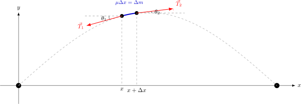
Consider a differential segment of an oscillating ideal string stretched along the x-axis. We examine a segment of length \Delta x with linear mass density \mu (kg/m) and constant tension T (N).

We assume the distortions of the string are small. This implies that the slope of the string is small everywhere, so the local angle \theta between the string and the horizontal is always small.

Figure 1: Differential segment of an ideal string under tension.

To find the equation of motion, we analyze the vertical forces acting on the segment between x and x + \Delta x. The net vertical force F_y is the difference between the vertical components of the tension at the two ends. Since there is no horizontal motion, the horizontal component of the tension is constant. For small angles (\cos \theta \approx 1), this implies the magnitude of the tension T is effectively constant throughout the segment, thus giving us the relation:

\begin{align*} F_y &= T \sin(\theta(x + \Delta x)) - T \sin(\theta(x)) \\ &= T \sin(\theta_2) - T \sin(\theta_1) \end{align*}

We can then use the small angle approximation, where the sine of the angle is approximately equal to its tangent (\sin \theta \approx \tan \theta).

Geometrically, the tangent of the angle represents the instantaneous slope of the string:

\sin(\theta) \approx \tan(\theta) = \frac{\partial y}{\partial x}

Substituting this approximation back into the force equation allows us to express the forces in terms of the string’s slope rather than trigonometric angles:

F_y \approx T \left[ \frac{\partial y}{\partial x}\bigg|_{x+\Delta x} - \frac{\partial y}{\partial x}\bigg|_{x} \right]

We apply Newton’s Second Law (F = ma) to the segment and define the following:

• Mass (m): The mass of the segment is \mu \Delta x.
• Acceleration (a): The vertical acceleration is \frac{\partial^2 y}{\partial t^2}.

Resulting in the equation:

T \left[ \frac{\partial y}{\partial x}\bigg|_{x+\Delta x} - \frac{\partial y}{\partial x}\bigg|_{x} \right] = (\mu \Delta x) \frac{\partial^2 y}{\partial t^2}

To isolate the spatial terms, we divide the entire equation by \Delta x:

T \left[ \frac{ \frac{\partial y}{\partial x}\big|_{x+\Delta x} - \frac{\partial y}{\partial x}\big|_{x} }{\Delta x} \right] = \mu \frac{\partial^2 y}{\partial t^2}

Now, we take the limit as the segment length approaches zero. The term in the brackets matches the fundamental definition of the derivative (see Definition 1). In our case, the function being differentiated is the slope, \frac{\partial y}{\partial x}. Therefore, the limit yields the derivative of the slope, which is the second spatial derivative:

\lim_{\Delta x \to 0} \left[ \frac{ \frac{\partial y}{\partial x}\big|_{x+\Delta x} - \frac{\partial y}{\partial x}\big|_{x} }{\Delta x} \right] = \frac{\partial}{\partial x}\left( \frac{\partial y}{\partial x} \right) = \frac{\partial^2 y}{\partial x^2}

This results in the PDE:

T \frac{\partial^2 y}{\partial x^2} = \mu \frac{\partial^2 y}{\partial t^2}

Rearranging the equation above highlights the physical mechanism of wave propagation:

\frac{\partial^2 y}{\partial t^2} = \frac{T}{\mu} \frac{\partial^2 y}{\partial x^2}

This equation states that acceleration is proportional to curvature.

• Zero Curvature: If the string is a straight line (constant slope), \frac{\partial^2 y}{\partial x^2} = 0. The tension vectors at x and x+\Delta x are parallel and cancel perfectly. The net force is zero, so the string does not accelerate.
• Non-Zero Curvature: When the string curves, the tension vectors are misaligned. While their horizontal components cancel, their vertical components sum to create a net restoring force.

The string curves specifically to generate the force required to accelerate the mass back toward equilibrium. This interaction causes the disturbance to propagate.

Finally, to reach the standard form, we define the propagation velocity v:

v = \sqrt{\frac{T}{\mu}}

Substituting this into our equation, we arrive at the classical 1D wave equation:

Definition 1 Recall the definition of the derivative: f'(x) = \lim_{h \to 0} \frac{f(x+h) - f(x)}{h}

\frac{\partial^2 y}{\partial t^2} = v^2 \frac{\partial^2 y}{\partial x^2} where:

• y(x,t) is the vertical displacement of the string at position x and time t.
• v= \sqrt{\frac{T}{\mu}} is the wave speed along the string.

The equation shows that the acceleration \left(\frac{\partial^2 y}{\partial t^2}\right) of any point on the string is proportional to its curvature² \left(\frac{\partial^2 y}{\partial x^2}\right).This makes intuitive sense. The more curved the string is, the stronger the net restoring force from the string’s tension, which in turn creates a greater acceleration, pulling it back toward its equilibrium position. So,a higher tension T or a lower mass density \mu results in a faster wave propagation speed c, and thus a higher frequency of the string.

² Curvature, also referred to as concavity

viewof curvature = Inputs.range([-1.0, 1.0], {
  value: -0.8, 
  step: 0.1, 
  label: "Initial Curvature"
})

// We give the container an ID so we can strictly attach the button to it
container_stable_v4 = html`<div id="sim-container" style="
  position: relative; 
  width: 100%; 
  max-width: 700px;
  height: 350px; 
  border: 1px solid var(--sim-border); 
  border-radius: 8px;
  overflow: hidden; /* Keeps button inside corners */
"></div>`

p5 = require("p5@1.9.0")

{
  const sketch = (s) => {
    let nodes = [];
    let numNodes = 40;  
    
    // --- STABILITY SETTINGS ---
    let subSteps = 8;       // Calculate physics 8 times per frame for smoothness
    let tension = 0.1;      // "Snappiness" of the string
    let damping = 0.999;     // Energy loss (prevents wobbling forever)
    let maxVelocity = 0.5;  // CRITICAL FIX: The Speed Limit. Prevents explosions.
    
    let isRunning = false;
    let btn;

    // Helper to get theme colors dynamically
    function getThemeColors() {
      let style = getComputedStyle(document.body);
      return {
        bg: style.getPropertyValue('--sim-bg').trim() || '#ffffff',
        stroke: style.getPropertyValue('--sim-stroke').trim() || '#1e1e1e',
        text: style.getPropertyValue('--sim-text').trim() || '#323232',
        accent: style.getPropertyValue('--sim-accent').trim() || '#00cc00'
      };
    }

    s.setup = () => {
      let c = s.createCanvas(700, 350);
      
      // --- BUTTON (Top Right of Container) ---
      btn = s.createButton('RELEASE');
      btn.parent(container_stable_v4); 
      
      // Force button to Top-Right corner
      btn.style('position', 'absolute');
      btn.style('top', '15px');
      btn.style('right', '15px');
      btn.style('z-index', '10');
      
      btn.mousePressed(toggleSimulation);
      styleButton(btn, false);
      
      resetString();
    };

    function resetString() {
      nodes = [];
      isRunning = false;
      if(btn) styleButton(btn, false);
      
      let curveAmount = -1 * curvature; 
      
      for (let i = 0; i < numNodes; i++) {
        let x = s.map(i, 0, numNodes - 1, -1, 1);
        
        // Initial Shape: Parabola 
        // We use a gentle curve formula to prevent starting with "broken" physics
        let y = curveAmount * (x * x - 1) * 0.8; 
        
        nodes.push({
          y: y, 
          v: 0,
          fixed: (i === 0 || i === numNodes - 1)
        });
      }
    }

    function toggleSimulation() {
      if (isRunning) {
        resetString();
      } else {
        isRunning = true;
        styleButton(btn, true);
      }
    }

    function styleButton(b, running) {
      // Use CSS variables for the button so it adapts to theme
      if(running) {
        b.html("RESET");
        b.style('background-color', 'var(--sim-bg)');
        b.style('border', '2px solid #ff4444');
        b.style('color', '#ff4444');
      } else {
        b.html("RELEASE");
        b.style('background-color', 'var(--sim-bg)');
        b.style('border', '2px solid var(--sim-accent)');
        b.style('color', 'var(--sim-accent)');
      }
      b.style('padding', '8px 16px');
      b.style('border-radius', '4px');
      b.style('cursor', 'pointer');
      b.style('font-weight', 'bold');
      b.style('font-family', 'system-ui, sans-serif');
      b.style('box-shadow', '0 2px 4px rgba(0,0,0,0.1)');
    }

    s.draw = () => {
      let colors = getThemeColors();
      s.background(colors.bg);
      
      // --- PHYSICS ENGINE ---
      if (isRunning) {
        for(let k=0; k<subSteps; k++){
          // Pass 1: Update Velocities
          for (let i = 0; i < numNodes; i++) {
              if(nodes[i].fixed) continue;
              
              let prev = nodes[i - 1];
              let curr = nodes[i];
              let next = nodes[i + 1];
              
              // 1. Calculate Force (Curvature)
              let force = (prev.y - 2 * curr.y + next.y);
              
              // 2. Update Velocity
              let accel = force * tension;
              curr.v += accel;
              curr.v *= damping;
              
              // 3. Safety Clamp
              curr.v = s.constrain(curr.v, -maxVelocity, maxVelocity);
          }

          // Pass 2: Update Positions
          for (let i = 0; i < numNodes; i++) {
            if(!nodes[i].fixed) {
              nodes[i].y += nodes[i].v;
            }
          }
        }
      }

      // --- RENDER ---
      
      // 1. Draw The String
      s.noFill();
      s.stroke(colors.stroke);
      s.strokeWeight(4);
      s.beginShape();
      for (let i = 0; i < numNodes; i++) {
        let px = s.map(i, 0, numNodes-1, 50, s.width - 50);
        // Scale Y for visibility (150x zoom)
        let py = s.height/2 + (nodes[i].y * 150); 
        s.vertex(px, py);
      }
      s.endShape();
      
      // 2. Draw HUD & Arrow
      drawHUD(s, colors);
    };
    
    function drawHUD(s, colors) {
      let centerIdx = Math.floor(numNodes / 2);
      let cNode = nodes[centerIdx];
      let lNode = nodes[centerIdx - 1];
      let rNode = nodes[centerIdx + 1];

      // Calculate logic values for display
      let rawCurve = (lNode.y - 2 * cNode.y + rNode.y);
      let displayCurve = -1 * rawCurve * 100; // Human readable scale
      let displayAccel = displayCurve * 2.0; 

      // Arrow Position
      let cx = s.width / 2;
      let cy = s.height / 2 + (cNode.y * 150);
      
      // Draw Arrow if there is acceleration
      // We check > 0.01 to ensure it shows even for static curvature
      if (s.abs(displayAccel) > 0.01) {
          let arrowLen = -displayAccel * 60; 
          // Clamp visual arrow size so it doesn't cover the text
          arrowLen = s.constrain(arrowLen, -150, 150);
          
          drawArrow(s, cx, cy, 0, arrowLen, '#ff3333');
      }

      // Text Info
      s.noStroke();
      s.fill(colors.text);
      s.textSize(14);
      s.textAlign(s.LEFT, s.TOP);
      s.textStyle(s.BOLD);
      s.text("String Physics", 20, 20);
      s.textStyle(s.NORMAL);
      s.fill(colors.text); // Use text color instead of hardcoded gray
      s.text(`Curvature: ${displayCurve.toFixed(2)}`, 20, 45);
      
      // For acceleration, we keep the green/red but make them slightly brighter/adaptive if we wanted? 
      // For now, let's stick to the conditional logic but maybe use safer colors
      s.fill(displayAccel > 0 ? '#00cc00' : '#ff4444'); 
      s.text(`Acceleration: ${displayAccel.toFixed(2)}`, 20, 65);
    }
    
    function drawArrow(s, x, y, vx, vy, color) {
      s.push();
      s.stroke(color);
      s.fill(color);
      s.strokeWeight(3);
      s.translate(x, y);
      s.line(0, 0, vx, vy);
      s.translate(vx, vy);
      s.rotate(s.atan2(vy, vx));
      s.triangle(0, 0, -6, 3, -6, -3);
      s.pop();
    }
  };

  // --- CLEANUP ---
  if (window.p5_sim_final) {
    window.p5_sim_final.remove();
  }
  let myp5 = new p5(sketch, container_stable_v4);
  window.p5_sim_final = myp5;
  invalidation.then(() => myp5.remove());
}

Solution to the Wave Equation: Harmonics ■

The solution to this wave equation, for a string fixed at both ends (e.g., at x=0 and x=L), is a superposition of standing waves, known as harmonics or partials. The general solution is a Fourier series:

TipDerivation

To find the solution to the wave equation, we will start with the assumption that the PDE is separable³ as a way to isolate the space and time variables. We assume a trial solution of the form:

y(x, t) = X(x)T(t)

We substitute this into the wave equation and separate the variables to find the solutions for X(x) and T(t).

T(t)X^{\prime\prime}(x) = \frac{1}{c^2} T^{\prime\prime}(t)X(x)

Dividing both sides by X(x)T(t), we obtain:

\frac{X^{\prime\prime}(x)}{X(x)} = \frac{1}{c^2} \frac{T^{\prime\prime}(t)}{T(t)}

Since the left side depends only on x and the right side depends only on t, both sides must be equal to a constant (see Lemma 1). We will call this constant -k^2 (to ensure oscillatory solutions and not exponential growth, we set the constant to be negative). This leads to two ordinary differential equations (ODEs):

\mathbf{Space}: X^{\prime\prime}(x) + k^2 X(x) = 0

\mathbf{Time}: T^{\prime\prime}(t) + k^2 c^2 T(t) = 0

These are standard harmonic oscillator equations. Their solutions are:

X(x) = C_1 \cos(k x) + C_2 \sin(k x)

T(t) = C_3 \cos(\omega t) + C_4 \sin(\omega t)

where \omega = k c is the angular frequency.

Now since we assume the string is fixed at both ends, we apply the boundary conditions y(0,t) = 0 and y(L,t) = 0 and can solve for the constants of the spacial part (i.e. C_1 and C_2).

\begin{align} \text{At } x&=0:\ C_1 \cos(0) + C_2 \sin(0) = 0 \implies C_1 = 0 \\ \text{At } x&=L:\ C_2 \sin(k L) = 0 \end{align}

For non-trivial solutions, B \neq 0, the sine term must be zero. Sine being zero implies that k must be discrete, i.e. 

k_n = \frac{n\pi}{L} \quad\mathbf{for}\ n = 1, 2, 3, ...

Thus the solution for X(x) is:

X(x) = \sin\left(k_n x\right)

(We will drop the constant coefficient here (e.g. C_2) and absorb it into the complete solution)

Recalling our assumption: y(x, t) = X(x)T(t), we can combine our solutions (and our constant coefficients) to yield the complete solution:

\begin{aligned} y_n(x,t) &= X_n(x) \cdot T_n(t) \\ y_n(x,t) &= \underbrace{\sin(k_n x)}_{\text{Shape on the string}} \cdot \underbrace{[A_n \cos(\omega_n t) + B_n \sin(\omega_n t)]}_{\text{Oscillation over time}} \end{aligned}

With this solution, we can make a few observations:

• X_n(x) (The Spatial Profile): Because this term has no t variable, the points where the string is still (the nodes) and where it reaches maximum displacement (the antinodes) are fixed in space, thus dictating the “geometry” of the wave.
• T_n(t) (The Temporal Scaling): Dependent on time, this term doesn’t change the relative shape of the string; instead, it tells every point on that X_n(x) stencil exactly what percentage of its maximum height it should be at any given moment. It forces the Spatial Profile to expand, flatten, and flip across the equilibrium line periodically.

However, since the wave equation is linear, the general solution is a superposition of all valid n modes. This superposition yields the Fourier series solution:

y(x, t) = \sum_{n=1}^{\infty} \sin\left(\frac{n\pi x}{L}\right) \left[A_n\cos\left(\omega_n t\right) + B_n\sin\left(\omega_n t\right)\right]

Where:

• \sin\left(\frac{n\pi x}{L}\right) represents the standing wave shape (harmonics).
• The terms in the bracket represent the oscillation in time.
• A_n and B_n are Fourier coefficients determined by the initial shape and velocity of the string.

Expanding all terms, we get:

³ One may ask how we could just assume that the PDE is separable. In reality, we are hoping that we are lucky and that the assumption holds after we finish solving the PDE. Most PDEs are not separable, and finding a solution to a non-separable PDE is often a very complex task.

Lemma 1 (Argument of separation of variables:) Imagine a the system: L(x) = R(t) Where x and t are independent variables. To prove L(x) is constant, we differentiate both sides with respect to x: \frac{\partial}{\partial x} \left[ L(x) \right] = \frac{\partial}{\partial x} \left[ R(t) \right] Since R(t) is a function of t only, it is treated as a constant with respect to x. Therefore, the derivative is zero L(t)^{\prime} = 0 and \therefore L(x) = C for some constant C. If you differentiate the system with respect to t, the same logic applies and R(t) = C and given how L(x) = R(t), they both equal the same constant L(x) = R(t) = C

y(x, t) = \sum_{n=1}^{\infty} \sin\left(\frac{n\pi x}{L}\right) \left[A_n\cos\left(\frac{n\pi c t}{L}\right) + B_n\sin\left(\frac{n\pi c t}{L}\right)\right]

Each term in the series represents a mode of vibration with a specific frequency:

• Fundamental Frequency (n=1): f_1 = \frac{v}{2L} = \frac{1}{2L}\sqrt{\frac{T}{\mu}}. This is the lowest frequency and determines the pitch we perceive⁴.
• Overtones (n>1): f_n = n\cdot f_1. These are integer multiples of the fundamental frequency.

⁴ Recall that wavelength is defined as \lambda = \frac{v}{f} with the wavelength of the fundamental being \lambda_1 = 2L.

TipWhat does “solution” mean physically?

When we say we have “solved” the PDE and found y(x,t), what do we actually possess?

Mathematically, the function y(x,t) is a tool that we can use to calculate the displacement of the string at any point in space and time.

• Without this, we would only know the behavior that the string would follow (e.g. Newton’s laws and the Wave equation).
• With this, we know the outcome of the system, making it deterministic.

Physcially, y(x,t) is a surface in 3D space.

• If you slice this surface at a fixed time t_0, the cross-section y(x, t_0) is a photograph of the string’s shape at that moment.
• If you slice this surface at a fixed position x_0, the cross-section y(x_0, t) is a history graph of that single particle’s motion up and down.

In summary, the solution is not just the physics but also its environment and conditions

• The terms inside the PDE (\frac{\partial^2}{\partial x^2}) encode the fundamental laws (Force = Mass \times Acceleration).
• The restrictions on the constants (n\pi/L) encode the geometry (the string is tied down).
• The coefficients (A_n, B_n) encode the history (how you plucked the string).

Timbre

Why is this important to piano tuning?

Well the timbre, or unique sound quality, of the piano note is determined by the relative amplitudes (A_n) of these harmonics. The hammer’s shape, hardness, and striking position excite these harmonics with different initial energies, creating the piano’s characteristic rich and complex tone.

Below is an interactive simulation of how the relative amplitudes of the harmonics affect the timbre of a vibrating string. Adjust the sliders to see how the timbre changes. Keep in mind that simulation does not capture the visual change of the fundamental frequency but rather, only the relative amplitudes of the harmonics.

// Container for the P5 sketch
container_harmonics = html`<div id="harmonics-sim" style="
  position: relative; 
  width: 100%; 
  max-width: 700px;
  height: 350px; 
  border: 1px solid var(--sim-border); 
  border-radius: 8px;
  overflow: hidden;
  margin-bottom: 20px;
"></div>`

viewof params = Inputs.form({
  fund: Inputs.range([110, 880], {step: 1, value: 220, label: "Fundamental (Hz)"}),
  g1: Inputs.range([0, 1], {step: 0.01, value: 0.8, label: "1st Harmonic (Fund)"}),
  g2: Inputs.range([0, 1], {step: 0.01, value: 0.0, label: "2nd Harmonic"}),
  g3: Inputs.range([0, 1], {step: 0.01, value: 0.0, label: "3rd Harmonic"}),
  g4: Inputs.range([0, 1], {step: 0.01, value: 0.0, label: "4th Harmonic"}),
  g5: Inputs.range([0, 1], {step: 0.01, value: 0.0, label: "5th Harmonic"}),
  g6: Inputs.range([0, 1], {step: 0.01, value: 0.0, label: "6th Harmonic"})
}, {
  template: (inputs) => {
    // Helper to format rows
    // We bind the update logic to the fundamental slider
    const rows = [
      { id: 'g1', n: 1, label: '1st Harmonic' },
      { id: 'g2', n: 2, label: '2nd Harmonic' },
      { id: 'g3', n: 3, label: '3rd Harmonic' },
      { id: 'g4', n: 4, label: '4th Harmonic' },
      { id: 'g5', n: 5, label: '5th Harmonic' },
      { id: 'g6', n: 6, label: '6th Harmonic' }
    ];

    // Create spans for frequencies
    const spans = {};
    rows.forEach(r => {
        spans[r.id] = html`<span style="font-family: monospace; font-weight: bold; margin-left: 10px; min-width: 60px;"></span>`;
    });

    const updateFreqs = () => {
       // inputs.fund is the DOM element returned by Inputs.range
       // Its value property is the current number
      const f = inputs.fund.value; 
      
      rows.forEach(r => {
           const val = f * r.n;
          spans[r.id].textContent = `${val} Hz`;
      });
    };

    // Listen to fundamental changes
    // Inputs.range triggers 'input' events on itself (it's a wrapper, but usually bubbles or dispatches)
    // Standard OJS inputs dispatch 'input' on the returned element.
    inputs.fund.addEventListener('input', updateFreqs);
    
    // Initial update (defer slightly to ensure value is ready if needed, currently direct access works)
    updateFreqs();

    // Build the grid
    // We want the slider and the frequency side-by-side
    // inputs.g1 is the slider element including its label (because we set label: "...")
    // Actually, Inputs.range with label creates a label > input structure.
    // To append text to the right, we might need to wrap them in a flex row.
    
    return html`<div style="display: flex; flex-direction: column; gap: 5px; max-width: 600px;">
      <div style="margin-bottom: 10px;">${inputs.fund}</div>
      ${rows.map(r => html`<div style="display: flex; align-items: center;">
          <div style="flex: 1;">${inputs[r.id]}</div>
          ${spans[r.id]}
      </div>`)}
    </div>`;
  }
})

{
  const sketch = (s) => {
    // --- AUDIO CONTEXT ---
    let audioCtx;
    let oscillators = [];
    let masterGain;
    let isPlaying = false;
    let btn;
    
    // Config
    const numHarmonics = 6;
    
    // Helper to get theme colors dynamically
    function getThemeColors() {
      let style = getComputedStyle(document.body);
      return {
        bg: style.getPropertyValue('--sim-bg').trim() || '#ffffff',
        stroke: style.getPropertyValue('--sim-stroke').trim() || '#1e1e1e',
        text: style.getPropertyValue('--sim-text').trim() || '#323232',
        accent: style.getPropertyValue('--sim-accent').trim() || '#00cc00'
      };
    }
    
    // Data from inputs (closure)
    // We will read the latest values in the draw/audio loop or reactively update
    
    s.setup = () => {
      let c = s.createCanvas(700, 350);
      
      // Play Button
      btn = s.createButton('PLAY SOUND');
      btn.parent(container_harmonics); 
      btn.style('position', 'absolute');
      btn.style('top', '15px');
      btn.style('right', '15px');
      btn.style('z-index', '10');
      btn.mousePressed(toggleAudio);
      styleButton(btn, false);
    };

    function startAudio() {
      if (!audioCtx) {
        audioCtx = new (window.AudioContext || window.webkitAudioContext)();
        masterGain = audioCtx.createGain();
        masterGain.gain.setValueAtTime(0.3, audioCtx.currentTime); // Master volume
        masterGain.connect(audioCtx.destination);
        
        // Create Oscillators
        for(let i=0; i<numHarmonics; i++) {
          let osc = audioCtx.createOscillator();
          let gain = audioCtx.createGain();
          osc.connect(gain);
          gain.connect(masterGain);
          osc.start();
          oscillators.push({osc, gain});
        }
      }
      if(audioCtx.state === 'suspended') {
        audioCtx.resume();
      }
      masterGain.gain.cancelScheduledValues(audioCtx.currentTime);
      masterGain.gain.setValueAtTime(0.3, audioCtx.currentTime);
    }
    
    function stopAudio() {
        if(masterGain) {
            masterGain.gain.setValueAtTime(masterGain.gain.value, audioCtx.currentTime); 
            masterGain.gain.exponentialRampToValueAtTime(0.0001, audioCtx.currentTime + 0.1);
        }
        // distinct from "suspending", we just mute it to effectively stop
    }

    function toggleAudio() {
        if(!isPlaying) {
            startAudio();
            isPlaying = true;
            styleButton(btn, true);
        } else {
            stopAudio();
            isPlaying = false;
            styleButton(btn, false);
        }
    }

    function styleButton(b, running) {
      if(running) {
        b.html("STOP");
        b.style('background-color', 'var(--sim-bg)');
        b.style('border', '2px solid #ff4444');
        b.style('color', '#ff4444');
      } else {
        b.html("PLAY SOUND");
        b.style('background-color', 'var(--sim-bg)');
        b.style('border', '2px solid var(--sim-accent)');
        b.style('color', 'var(--sim-accent)');
      }
      b.style('padding', '8px 16px');
      b.style('border-radius', '4px');
      b.style('cursor', 'pointer');
      b.style('font-weight', 'bold');
      b.style('font-family', 'system-ui, sans-serif');
    }

    s.draw = () => {
      let colors = getThemeColors();
      s.background(colors.bg);
      
      // Update Audio Params
      // Note: In OJS, 'fundamental', 'gain1', etc are available in scope if we pass them
      // But to ensure we get the *latest* reactive check, typical OJS+P5 pattern is slightly different
      // We'll rely on the reactive cell structure re-calling these or 
      // effectively we can read them from window if we attached them?
      // ACTUALLY: The P5 cell will re-run if inputs change unless we use a closure. 
      // BUT re-running setup() kills the audio context.
      // TRICK: We will pass values via a global object or update a property on the sketch object
      // OR we assume update logic happens outside?
      
      // BETTER PATTERN for OJS P5:
      // The variables 'fundamental', 'gain1' etc are available in this expected scope
      // because this block will be re-evaluated when they change? 
      // NO, if we put the whole thing in a block, it re-inits on change.
      // We need the sketch to persist and values to be injected.
      
      // We will look for an updateValues method we attach to the canvas element or similar?
      // No, simplest way in Quarto OJS: use a mutable object or just read the values 
      // if we are in the same scope. 
      
      // However, to prevent re-initialization of audio context, we need to NOT re-run this cell
      // whenever 'fundamental' changes.
      // We do this by... NOT referencing `fundamental` directly in the definition.
      // Instead we use a mutable or a secondary cell to push updates.
      
      // Let's assume we use `window.harmonics_params` as a bridge if needed, 
      // or just `s.harmonics_params` and update it from another cell.
      
      const params = window.harmonics_params || {f: 220, gains: [0,0,0,0,0,0]};
      
      if(video_audio_active && isPlaying && audioCtx) {
          updateAudioOscillators(params);
      }
      
      // Draw Waveform
      drawWaveform(s, params, colors);
    };
    
    let video_audio_active = true; // Gate
    
    function updateAudioOscillators(p) {
        if(!audioCtx) return;
        const f = p.f;
        const g = p.gains;
        
        const now = audioCtx.currentTime;
        
        for(let i=0; i<numHarmonics; i++) {
            let oscObj = oscillators[i];
            if(!oscObj) continue;
            
            // Frequency = f * (i+1)
            // We use linear ramp for smooth pitch slide
            oscObj.osc.frequency.setTargetAtTime(f * (i+1), now, 0.05);
            
            // Gain
            oscObj.gain.gain.setTargetAtTime(g[i] * 0.3, now, 0.05); // * 0.3 to prevent clipping sum
        }
    }

    function drawWaveform(s, p, colors) {
        s.stroke(colors.stroke);
        s.strokeWeight(2);
        s.noFill();
        
        s.beginShape();
        const w = s.width;
        const h = s.height;
        const cy = h / 2;
        
        // Show ~2 cycles of fundamental
        // T = 1/f. Width represents time? 
        // Let's just visualize the pure shape: sum(Ai * sin(i * x))
        
        for(let x = 0; x < w; x+=2) {
            // Map x to phase 0..4PI (2 cycles)
            let phase = s.map(x, 0, w, 0, s.TWO_PI * 2);
            let yVal = 0;
            
            // Additive Synthesis
            for(let i=0; i<numHarmonics; i++) {
                let n = i + 1;
                let amp = p.gains[i];
                yVal += amp * s.sin(n * phase);
            }
            
            // Normalize visual height? 
            // Max potential amp is sum(gains). Let's scale reasonably.
            let yPx = cy - (yVal * 50); 
            s.vertex(x, yPx);
        }
        s.endShape();
        
        // Info text
        s.noStroke();
        s.fill(colors.text);
        s.text(`Freq: ${p.f} Hz`, 10, h - 20);
    }
  };

  // --- CLEANUP ---
  if (window.p5_harmonics) {
    window.p5_harmonics.remove();
    // Maybe close audio context too?
    // window.harmonics_ctx.close();
  }
  
  let myp5 = new p5(sketch, container_harmonics);
  window.p5_harmonics = myp5;
  invalidation.then(() => {
      myp5.remove();
       // We probably want to stop audio if cell re-runs
  });
}

{
  window.harmonics_params = {
      f: params.fund,
      gains: [params.g1, params.g2, params.g3, params.g4, params.g5, params.g6]
  };
}

ImportantReal Piano timbre

In reality real piano strings are stiff, not perfectly flexible. This stiffness adds a restoring force, slightly altering the frequencies of the overtones. They become slightly sharper (higher in frequency) or flatter (lower in frequency) than perfect integer multiples of the fundamental. This phenomenon, known as inharmonicity, is a key characteristic of the piano’s sound.

This will be properly covered in the end of the document

The Soundboard: String amplification

While we modeled the string ends as fixed points to derive the frequencies, in reality, the piano bridge end moves microscopically—this ‘imperfection’ in the boundary condition is exactly how energy escapes the string to reach your ears.

A vibrating string on its own displaces very little air and produces a very faint sound. To make the sound audible, its energy must be transferred to a larger radiating surface. This is the job of the soundboard.

Figure 2: Upright Piano String and Soundboard

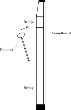
The strings are stretched over a wooden bridge, which is glued directly to a large, thin sheet of wood (typically spruce)—the soundboard. The strings’ vibrations travel through the bridge, forcing the entire soundboard to vibrate. Because the soundboard has a much larger surface area than the strings, it can move a significant volume of air, thus acting as an efficient acoustic amplifier. It doesn’t add energy, but rather converts the string’s vibrational energy into audible sound energy more effectively.

Acoustic Wave Propagation ■ / ■

The vibrating soundboard acts like a large piston, creating compressions and rarefactions (areas of high and low pressure) in the surrounding air. These pressure disturbances propagate outward as a sound wave.

TipSupplemental Material

If you are interested in how to simulate acoustic behavior with FDTD , you can find it in the supplemental material section.

The Acoustic Wave Equation ■

The propagation of sound in a medium like air is described by the three-dimensional acoustic wave equation:

TipDerivation

To begin, we will start with the following assumptions:

• We treat air not as discrete particles, but as a continuous fluid.
• We assume the disturbance is a “small signal” (linear behavior), meaning the fluctuations are tiny compared to the static atmospheric values.

We will also identity our unknown variables as follows:

• Pressure (P): Total pressure P(\vec{r}, t) = P_0 + p(\vec{r}, t), where P_0 is static atmospheric pressure and p is the acoustic pressure.
• Density (\rho): Total density \rho(\vec{r}, t) = \rho_0 + \rho'(\vec{r}, t), where \rho_0 is static atmospheric density and \rho' is the acoustic density fluctuation.
• Particle Velocity (\vec{u}): The velocity of the fluid elements \vec{u}(\vec{r}, t). Ambient air velocity is assumed to be zero.

To solve for the three unknown variables (p, \rho', \vec{u}), we require three independent physical laws. These are presented in their linearized forms, assuming small perturbations where second-order terms (like convective acceleration) are negligible.

The Linearized Continuity Equation (Conservation of Mass)

This equation relates the scalar density field to the vector velocity field.

\frac{\partial \rho'}{\partial t} + \rho_0 \nabla \cdot \vec{u} = 0

This is the differential form of mass conservation.

• Physically, it states that the time rate of change of the scalar mass density is exactly balanced by the negative divergence of the mass flux density vector (\vec{J}_m \approx \rho_0 \vec{u}). If the flux vector field has non-zero divergence (a source or sink, i.e \nabla \cdot \vec{u} \neq 0), the local density must change time-synchronously. In other words, this equation asserts that a non-zero divergence in the velocity field (local expansion or compression) must result in a corresponding time-rate change of the scalar density field.

The Linearized Euler’s Equation (Conservation of Momentum)

This is the fluid dynamic equivalent of Newton’s Second Law, neglecting viscous losses and convective acceleration terms. \rho_0 \frac{\partial \vec{u}}{\partial t} = -\nabla p

where:

• \nabla p represents the spatial variation of the pressure field.

• Physically, this equation couples the temporal change of the momentum density vector (\rho_0 \vec{u}) to the spatial variation of the pressure field. The negative gradient operator (-\nabla) implies that the acceleration vector of the fluid particles is aligned with the steepest descent of the scalar pressure field.

The Equation of State (Constitutive Relation)

Assuming an adiabatic process (negligible heat transfer during oscillation), we approximate the pressure-density relationship as linear. p = c^2 \rho'

• Physically, this provides the linear mapping between the two scalar fields (density and pressure), acting as the restoring force constant for the medium.

Derivation of the Acoustic Wave Equation

Our approach to derive the acoustic wave equation is to decouple the vector field \vec{u} from the scalar fields to form a single wave equation for pressure p(\vec{r},t).

Time-Differentiation of the Continuity Equation

We substitute the Equation of State (\rho' = p/c^2) into the Continuity Equation, then take the partial derivative with respect to time:

substitution \frac{1}{c^2} \frac{\partial p}{\partial t} + \rho_0 \nabla \cdot \vec{u} = 0

differentiation \frac{1}{c^2} \frac{\partial^2 p}{\partial t^2} + \rho_0 \frac{\partial}{\partial t} (\nabla \cdot \vec{u}) = 0

Since the spatial and temporal operators on continuous fields commute (\nabla \cdot \frac{\partial}{\partial t} = \frac{\partial}{\partial t} \nabla \cdot), we rewrite this as:

\frac{1}{c^2} \frac{\partial^2 p}{\partial t^2} + \rho_0 \nabla \cdot \left( \frac{\partial \vec{u}}{\partial t} \right) = 0

Divergence (Space-Differentiation) of Euler’s Equation

Next, we operate on Euler’s Equation with the divergence operator to isolate the term \nabla \cdot \frac{\partial \vec{u}}{\partial t}:

\nabla \cdot \left( \rho_0 \frac{\partial \vec{u}}{\partial t} \right) = \nabla \cdot (-\nabla p)

Applying the identity \nabla \cdot (\nabla \phi) = \nabla^2 \phi (the Laplacian), this becomes:

\rho_0 \nabla \cdot \left( \frac{\partial \vec{u}}{\partial t} \right) = -\nabla^2 p

Synthesis

We substitute the divergence of the acceleration term into the modified Continuity Equation

\frac{1}{c^2} \frac{\partial^2 p}{\partial t^2} + (-\nabla^2 p) = 0

Rearranging yields the homogeneous Acoustic Wave Equation:

\nabla^2 p - \frac{1}{c^2} \frac{\partial^2 p}{\partial t^2} = 0

\frac{\partial^2 p}{\partial t^2} = c^2 \nabla^2 p

where:

• p(x,y,z,t) is the acoustic pressure—the deviation from the ambient atmospheric pressure.
• c is the speed of sound in the medium (approximately 343 m/s in air at room temperature).
• \nabla^2 = \frac{\partial^2}{\partial x^2} + \frac{\partial^2}{\partial y^2} + \frac{\partial^2}{\partial z^2} is the Laplace operator, representing the spatial variation of pressure in all three dimensions.

This equation describes how a pressure change at one point in space spreads outwards spherically over time. The soundboard’s complex vibrations, containing all the harmonic frequencies from the strings, are imprinted onto this pressure wave.

Solutions to the Wave Equation

While the scalar Wave Equation governs the system dynamics, the solution topology depends on the boundary conditions and source geometry.

The Plane Wave

For a wave propagating in a single direction (e.g., \hat{x}), we assume invariance in y and z. The Laplacian reduces to \partial^2/\partial x^2.Harmonic Solution:

p(x,t) = P_+ e^{j(\omega t - kx)}

where k = \omega/c is the wavenumber and the real part of this complex function is the physical pressure wave. This represents a uniform wavefront with constant energy density.

The Spherical Wave

For a point source, we utilize spherical coordinates. Assuming isotropic radiation (symmetry in \theta and \phi), the Laplacian is \nabla^2 = \frac{1}{r^2}\frac{\partial}{\partial r}(r^2 \frac{\partial}{\partial r}).Harmonic Solution:

p(r,t) = \frac{A}{r} e^{j(\omega t - kr)}

Physical Implication:Unlike the 1D string or Plane Wave where amplitude is conserved, the Spherical Wave solution contains a 1/r dependence. This geometric attenuation is required to satisfy conservation of energy: as the spherical wavefront area expands by r^2, the power density (Intensity) must decrease by 1/r^2, necessitating that the pressure field amplitude decreases by 1/r.

Conclusion

For our purposes we are going to assume that the piano is a point source radiating sound waves into a free field. However, when we recieve the sound, we will assume that it arrives at the microphone as a plane wave. This is a reasonable assumption if the distance between the piano and the microphone is much larger than the wavelength of the sound.

Finally, the piano’s case and the position of its lid (open or closed) play a role in reflecting and directing these sound waves, shaping the final sound that reaches the listener’s ear. The entire structure works in concert to transform a simple hammer strike into a rich, resonant musical tone.